1) Make the notebook
2) make sure the *.ipynb file
3) run the following command 'jupyter nbconvert –to html –template basic notebook_blog.ipynb notebook_blog.html'
4) open the *.html file in an editor, copy the text, and paste into 'text' tab of a new post
All posts by Conrad Schiff
Masked Scientific Arrays
Define a typical scientific array
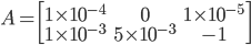
The definition of the matrix A is designed to represent a typical scientific data set that varies by orders of magnitude. In addition, some of the data is invalid due to either no measurement ( ) or there was a measurement glitch (
 ).
).
For sake of completeness, the entire matrix is given by:
In [16]:
A = np.array([[1e-4,0,1e-5],[1e-3,5e-3,-1]])
print A
A simple matrix plot (using matplotlib's pcolormesh) doesn't show anything useful since all the 'good' numbers are orders of magnitude smaller than the bad. Note also that the matrix is 'plotted up' as the zeroth row corresponds to the lowest row of the plot
In [17]:
plt.pcolormesh(A)
Out[17]:

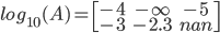
Of course, the way to bring out the data is by taking a logarithm - but the inclusion of the '0' and the '-1' are going to cause problems. Numpy gives two warnings (different ones) and it comes back with different values. The resulting matrix should look like
In [20]:
log_A = np.log10(A)
print log_A
This helps a bit, but unfortunately the 'bad' values put in a false color that says something it shouldn't.
In [21]:
plt.pcolormesh(log_A,vmin=-6,vmax=-3)
Out[21]:

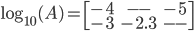
A much better alternative is to mark the bad points as invalid. Numpy's masked array does this for us. The correct invoccation is numpy.ma.masked_invalid, where ma is numpy's masked array package and masked_invalid is the function that takes care of $-\infty$ and $nan$. The proper array is now
In [22]:
masked_log_A = np.ma.masked_invalid(log_A)
print masked_log_A
In [23]:
plt.pcolormesh(masked_log_A,vmin=-6,vmax=-3)
Out[23]:

Smoothing Jupyter Startup
Within:
C:\Users\\.ipython\profile_default\startup
place whatever files you want executed with the following naming convention
00-global_imports.py
01-local_imports.py
02-global_magics.ipy
with contents like:
00-global_imports.py

#global imports
import matplotlib as mpl
mpl.use('agg')

import datetime          as dt
import matplotlib.cm     as cmap
import matplotlib.dates  as mdates
import matplotlib.pyplot as plt
import matplotlib.ticker as ticker
import numpy             as np
import os
import re
import scipy             as sp
import scipy.interpolate as interp
import scipy.optimize    as opt
import scipy.special     as special
import spacepy.pycdf     as pycdf
import sys
02-global_magics.ipy

#magic happens
%load_ext autoreload
%autoreload 2
%matplotlib inline
Block Quotations
- Common Cents
.myQuoteDiv {
background-color: #f5f5dc;
border-style: none;
border-left: 6px solid #d5d5bc;
width: 500px;
margin: 0px 0px 16px 50px;
padding: 4px 4px 4px 10px;
}
.myQuoteDiv .myAttrib {
margin-top: 8px;
font-style: italic;
}
<div class = "myQuoteDiv">Chipotle’s questionable marketing tactics, and similar recent marketing moves by Whole Foods and Panera, may have brought out the knives of scientists and science minded journalists, but they were not hatched in a vacuum. Consumers are responding to the demonization of GMOs and our foods are tainted with ‘dangerous’ chemicals.
<div class = "myAttrib">- Jon Entine & Rebecca Randall</div>
</div>
Making Nice Tables
table, th, td {
border: 1px solid black !important;
border-collapse: collapse !important;
color: black !important;
}
th { text-align: center !important;
background-color: #dee7d2 !important;}
Numerically solve an ODE in Maxima
As an example, solve the SHO numerically in Maxima
- load("dynamics")
- Specify only the RHS of
 . Note that dx_dt and dvx_dt are simply names of expressions
- dx_dt : vx
- dvx_dt : -omega^2 * x
- my_odes : [dx_dt,dvx_dt]
- Define the variable names
- var_names : [x,vx]
- Specify initial conditions
- x0 : 1
- vx0 : 0
- ICs : [x0,vx0]
- define the domain of time (independent variable name, span and step) over which the equations will be solved
- t_var : t
- t_start : 0
- t_stop : 10
- t_step : 0.1
- t_domain : [t_var, t_start, t_stop, t_step]
- Issue the command to run
- Z : rk(my_odes,var_names,ICs,t_domain)
Installing the LeatherDiary Theme
- Log into JustHost (not the WP admin on the client side but the admin on the server side)
- Locate the leatherdiary-premium directory under /public_html/wp-content/themes
- Locate the target subdomain (e.g. UnderTheHood)
- Copy the leatherdiary-premium directory whole from /public_html/wp-content/themes to /public_html/<subdomain>/wp-content/themes (e.g. the final directory structure for UnderTheHood would look like public_html/UnderTheHood/wp-content/themes/leatherdiary-premium)
- Now log into as WP admin on the subdomain side
- Goto 'Appearance' on the left widget
- Pick 'Themes' from there and then activate Leather Diary Premium
Changing the Appearance of the WordPress Installation
1) Log into subdomain on the WordPress side as ‘Admin’ (using pre-selected username and password – see Making a Subdomain)
2) From the left widget select 'Settings' (note that 'Settings' is only visible for 'Admin')
3) Under 'Settings' select:
- 'General' to change the Site Title and Tagline
- 'Writing' to change how posts appear, are categorized, or converted from email
- 'Reading' for how long posts stay active and how syndication and search engines work
- 'Discussion' for how the site manages comments, links from other sites, etc.
- 'Media' for how pictures are handled
- 'Permalinks' for how the style of permalinks is set
Posting
1) Log into the desired subdomain as Editor
2) On the left widget click on 'Posts'
3) Then click on 'Add New'
Setting up an Editor Account
1) Log into subdomain on the WordPress side as 'Admin' (using pre-selected username and password - see Making a Subdomain )
2) On the left widget go to 'Users' and select 'Add New'
3) Set username, email, and password as desired
4) Add the new user by clicking on 'Add New User'
5) If this is the first user account, find the 'Your site is currently showing the under construction page. To go live click here' banner near the top of the page and 'click there'
6) Log out of the WordPress instantiation